
Random Acts of Optimization
Game developers working on a continuously evolving product like League of Legends are constantly battling against the forces of entropy as they add more and more content into unfortunately finite machines. New content carries implicit cost—not just implementation cost but also memory and performance cost created by more textures, simulation, and processing. If we ignore (or miscalculate) that cost then performance degrades and League becomes less enjoyable. Hitches suck. Lag is infuriating. Frame rate drop is frustrating.
I'm part of a team dedicated to improving the performance of League of Legends. We profile both the client and the server, find problems (performance-related and otherwise), and then fix them. We also feed back what we’ve learned to other teams and provide them with the tools and metrics to identify their own performance problems before they affect players. We continually improve LoL's performance to open up space for artists and designers to add cool new stuff: we’re making it faster while they’re making it bigger and better.
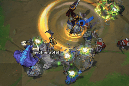
This is the first in a series about how as a team we optimize League of Legends while new content and fixes get continuously added. It’s an extremely rewarding challenge. This piece will dive into some interesting challenges we faced with the particle system—as you can see below particles play a major role in the game.
Optimization isn't simply rewriting a chunk of code in assembly—although sometimes it is that. We make changes that not only improve performance, but maintain correctness and, where possible, improve the state of the code. This last point is critical: any code that’s not readable and maintainable creates technical debt that we’d have to deal with later.
We take three basic steps when optimizing an existing codebase: identification, comprehension, and iteration.
Step 1: Identification
Before optimizing anything, we first confirm that the code needs optimization. There’s little benefit in optimizing what looks to be obviously slow code if it has minimal impact on overall performance. (Especially when that time and effort could be better spent elsewhere.) We use code instrumentation and sample profiling to help identify the non-performant sections of the codebase.
Step 2: Comprehension
Once we know which parts of the codebase are slow, we dive deeper into the code to really understand what’s going on. We need to know what the code does, as well as the intent of the original implementation. Then, we can figure out why this code is a bottleneck.
Step 3: Iteration
When we understand why the code is slow and what it’s supposed to do, we have enough information to devise and implement a possible solution. Using the instrumentation and profiling data from the identification step, we compare the performance of our new code against the old. If the solution’s fast enough and we’ve thoroughly tested it to ensure we haven’t introduced any new bugs, then it’s high fives all around, and we’re ready for further internal testing. In the more likely case that the code isn’t fast enough, we iterate on the solution until it is.
Let’s have a look at this process with respect to the League of Legends codebase and walk through a recent optimization of the particle system step-by-step.
Step 1: Identification
Riot engineers inspect the performance of the game client and server using a range of profiling tools. We first look at the client’s frame rate and high level profiling information (output via the instrumentation of selected functions) using Waffles, an in-house tool that allows us to communicate with internal builds of the client and server. (Additionally, Waffles can be used for many other things, such as triggering debug events for testing, inspecting in-game data like the navigation grid, and pausing or slowing down gameplay.)
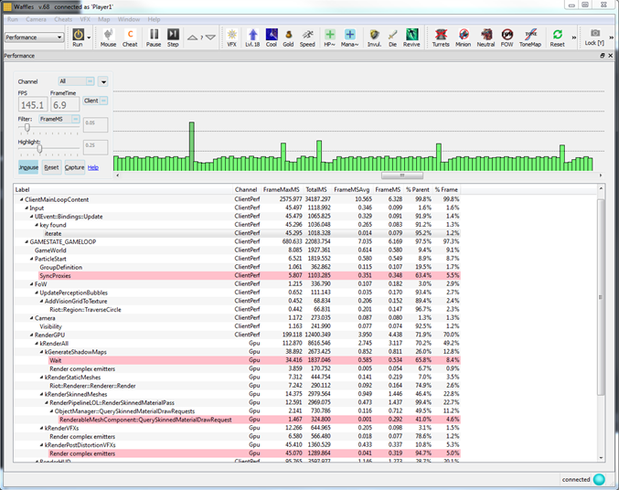
Waffles provides an interface to display live, detailed performance information. The image above shows how a typical example of client performance looks on it, with the top graph (green bars) representing the frame time in milliseconds—the higher the bar, the slower the frame. Very slow frames are noticeable as ‘hitches’ in gameplay. Below the graph is a hierarchical view of the important functions, where, by clicking any of the green bars, engineers receive an updated detailed breakdown of that frame. From there we can get a good indication of what section of the code is running slowly for that particular spike.
We use a simple macro to manually instrument important functions within the codebase to provide this performance-related information. For public builds the macro compiles out, but for profile builds it constructs a small class that creates an event that is pushed onto a large profile buffer. This event contains a string identifier, a thread ID, a timestamp, and any other information deemed necessary. (For example, it can store the number of memory allocations that have occurred within its lifetime.) When this object falls out of scope, the destructor updates the event in that buffer with the elapsed time since construction. At a later time, this profile buffer can be output and parsed—ideally in another process in order to minimize the impact to the game itself.
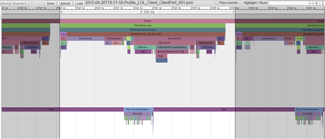
In our case we output the profile buffer to a file and read that into the visualization tool which is conveniently built into Chrome. (You can find more information about the tracing tool here and you can try it out by typing “chrome://tracing/” into your Chrome browser. It is designed for web page profiling, but the format of the input profile data is a simple json format that can be easily constructed from your own data.) From this we can see where there are slow functions, or where lots of small functions are called in sequence: both can be indications of suboptimal code.
Let me show you how: the view above is a typical Chrome Tracing view and shows two of the running threads on the client. The top one is the main thread, which does a majority of the processing, and the bottom one is the particle thread, which does particle processing. Each colored bar corresponds to a function, and the length of the bar indicates the time it takes to execute. Called functions are indicated by the vertical stacking—parents appear above children. This provides a fantastic way of visualizing the execution complexity as well as the time signature of the frame. When we spot an area with suboptimal code, we can zoom in on the particle section to see more detail on what’s happening.
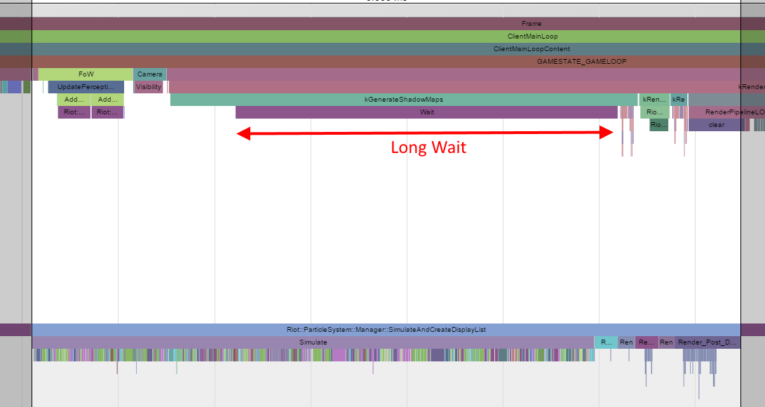
Let’s zoom in on the center portion of the graph. From the top thread we can see a very long wait that only ends when the particle Simulate function completes in the bottom thread. Simulate contains a large number of different function calls (the colored bars). Each of these is a particle system update function where the position, orientation, and other visible traits of each particle in that system are updated. One obvious optimization is to multithread the Simulate function to be run on the main thread as well as on the particle thread, but for this exercise we’ll look at optimizing the Simulate code itself.
Now that we know where we want to look for performance problems we can switch to sampling profiling. This type of profiling periodically reads and stores the program counter, and optionally the stack of the running process. After a period of time, this information gives a stochastic overview of where time was spent within the codebase. More samples will occur within the slower functions, and, even more usefully, the individual instructions that take the longest will also accrue more samples. In this we can see not only which functions are the slowest, but which lines of code are the slowest. There are many good sampling profilers available, from free ones like Very Sleepy to more fully-featured commercial ones like Intel’s VTune.
By running VTune on the game client and inspecting the particle thread, we can see a list of the slowest functions.
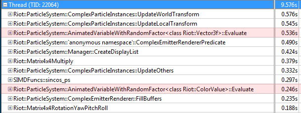
The table above shows a range of particle-related functions. For reference, the top two are fairly large functions that update a range of matrices and state related to position and orientation for each particle. For this example I’ll be looking at the Evaluate function in AnimatedVariableWithRandomFactor<> found at entries 3 and 9, because it is fairly small (and therefore easy to understand) yet comparatively costly.
Step 2: Comprehension
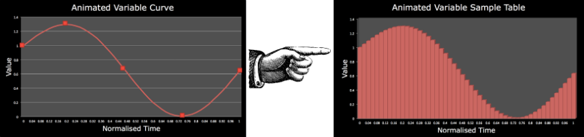
Now that we’ve picked a function to optimize we need to understand what it does and why. In this case, AnimatedVariables are used by LoL artists to define how particle traits change over time. After an artist specifies key-frame values for a particular particle variable, the code interpolates over that data to produce a curve. The interpolation method is either linear interpolation, or first- or second-order integration. Animation curves are used extensively — there are nearly 40,000 of them in Summoner’s Rift alone — for everything from particle color to scale to rotational velocity. The Evaluate() function is called hundreds of millions of times each game. Additionally, particles in LoL are a critical part of gameplay, and as such their behavior must not change at all.
This class had already been optimized to use a lookup table, an array that contains a precalculated value for each timestep, so the calculations could be reduced to just reading a value. This was a sensible choice as the first- and second-order integration of the curves is an expensive process. Performing that operation for every animated variable on every particle in every system would have resulted in significant slowdown.
When looking at a performance problem, it’s often helpful to exaggerate the problem by finding a worst case scenario. To simulate particle slowdown I set up a single player game with nine mid level bots and instigated a massive teamfight in the bottom lane. I then ran VTune over the client during this combat and recorded the various profile data. This gave the following sample attributions in the Evaluate code (shown below).
I’ve brought in lines 91-95 from the now commented out call to Evaluate on line 90 to make the situation easier to illustrate.
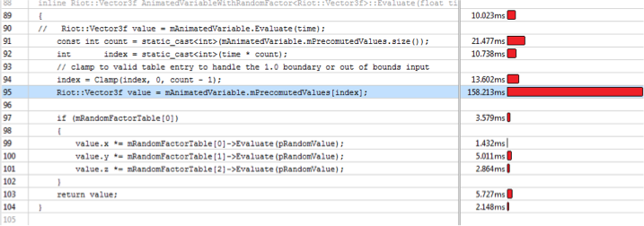
For those of you not familiar with VTune, this view shows the lines that samples were collected for during the profile run. The red bar to the right indicates the number of hits: the longer the bar, the more hits, and therefore the slower that line is. The time next to that bar is an approximation of the time spent processing that line. You can also bring up a view of the assembly for a particular function and see the exact instructions that are contributing to the slowdown.
If the big red bar is anything to go by, line 95 is the issue here. But all it’s doing is copying out a Vector3f from the incorrectly spelled look up table, so why is it the slowest part of this function? Why is a 12 byte copy so slow?
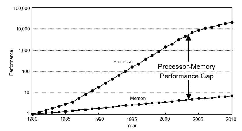
The answer lies in the way that modern CPUs access memory. CPUs have fairly reliably obeyed Moore’s Law and sped up by 60% per year, while memory speeds have languorously ambled along at a mere 10% per year.
Caching can mitigate this performance gap. Most of the CPUs League runs on have 3 caches: level 1 caches are the fastest but smallest, while level 3 are the slowest and largest. Reading data from the level 1 cache takes around 4 cycles while a read from main memory can take around 300 cycles or more. You can do a lot of processing in 300 cycles.
The problem with the initial lookup based solution is that while reading the values from the lookup table in order is pretty fast (due to hardware prefetching), the particles that we are processing are not stored in time order and so the lookups are effectively in random order. This often results in stalls while the CPU waits for data fetches from main memory. While 300 cycles is probably less than the cost of a first- or second-order integration we also need to know how often this is being used in the game.
To find out, a few quick additions to the code were made to collate the number and types of AnimatedVariables. They showed that out of the almost 38,000 AnimatedVariables:
- 37,500 were linearly interpolated; 100 were first order; and, 400 were second order.
- 31,500 had only one key; 2,500 had 3 keys; and, 1,500 had 2 or 4 keys.
So, the common path is for a single key. Since the code always generates a lookup table, this builds a table with a single value needlessly spread throughout it. This means that each look up (which always returns the same value) will generally cause a cache miss, resulting in a waste of memory and a waste of CPU cycles.
Very often, code becomes a bottleneck for one of four reasons:
- It’s being called too often.
- It’s a bad choice of algorithm: O(n^2) vs O(n), for example.
- It’s doing unnecessary work or it is doing necessary work too frequently.
- The data is bad: either too much data or the layout and access patterns are bad.
The problem here wasn’t with inadequate code design or implementation. The solution was good. But after extensive use by artists, the common path was for a single value, something that simply wouldn’t have been obvious during the implementation phase.
As an aside, one of the most important things I’ve learned as a programmer is to respect the code that you’re working on. The code may look crazy, but it was probably written that way for a very good reason. Don’t dismiss existing code as being stupid until you completely understand how it’s being used and what it was designed for.

Step 3:Iteration
Now we know where the slow code is, what it’s supposed to do, and why it’s slow. It’s time to start formulating a solution. Given that the most common execution path is for a single variable, we need to redesign the implementation with that in mind. We also know that the linear interpolation over a small number of keys is fast (simple calculations over small amounts of cache coherent data), so we need to consider that as well. Finally, we can drop back to the precomputed lookup in the rarer cases of integrated curves.
In the cases where we aren’t using the lookup table it makes no sense to construct that table in the first place, so this will free up significant amounts of memory. (Most of the tables were 256 entries in size or larger and each entry was up to 12 bytes in size which equates to around 3kb per table.) So we can now afford to use a little extra memory to add in a cached value of the number of entries and the single value that is being stored.
The original code’s data looked like this:
template <typename T>
class AnimatedVariable
{
    // <snip>
private:
    std::vector<float> mTimes;
    std::vector<T>     mValues;
};

template <typename T>
class AnimatedVariablePrecomputed
{
    // <snip>
private:
    std::vector<T> mPrecomutedValues;
};
The AnimatedVariablePrecomputed object was constructed from an AnimatedVariable object, interpolating and building a table of a specified size from it. Evaluate() was only ever called on the precomputed objects.
We changed the AnimatedVariable class to look like this:
template <typename T>
class AnimatedVariable
{
    // <snip>
private:
    int mNumValues;
    T mSingleValue;

    struct Key
    {
        float mTime;
        T     mvalue;
    };
    std::vector<Key> mKeys;
    AnimatedVariablePrecomputed<T> *mPrecomputed;
};
We’ve added a cached value, mSingleValue, and a number, mNumValues, to tell us when to use that value. If mNumValues is one (the single key case), Evaluate() will now simply immediately return mSingleValue—no further processing required. You'll also note interleaved the time and value vectors into a single vector to reduce cache misses.
Excluding the data the vectors point to the size of this class now ranges from 24 to 36 bytes depending on the template type (and depending on the platform, the size of std::vector<> can also vary).
The original Evaluate() method looked like this:
template <typename T>
T AnimatedVariablePrecomputed<T>::Evaluate(float time) const
{
    in numValues = mPrecomputedValues.size();
    RIOT_ASSERT(numValues > 1);

    int index = static_cast<int>(time * numValues);
    // clamp to valid table entry to handle the 1.0 boundary or out of bounds input
    index = Clamp(index, 0, numValues - 1);
    return mPrecomputedValues[index];
}
And our new Evaluate() method is below, shown in VTune. You can see the three possible execution cases: single value (red), linearly interpolated values (blue), and precomputed lookups (green).
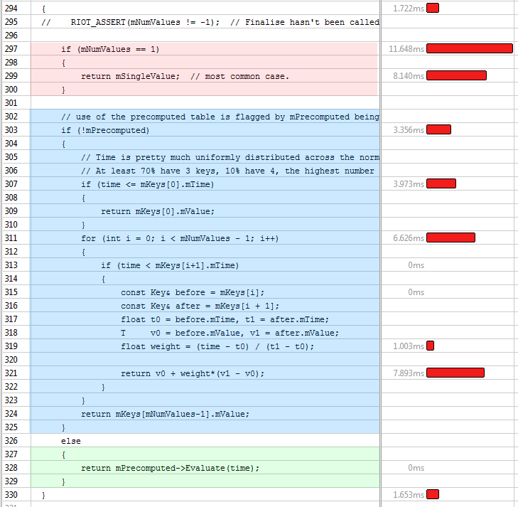
This new code runs roughly three times faster: the function now drops down from number 3 to number 22 in the list of slowest functions! And the best bit? It is not only faster, but it also uses less memory, about 750kb less. And, we’re not done yet! Not only is it faster and smaller, but it’s also more accurate for linearly interpolated values. Win, win, win.
What I’ve not shown here (as this post is already long enough) is the iterations that I went through to get to this solution. One of my first attempts was to reduce the size of the sample tables based on the lifetime of the particles. This mostly worked - but some of the faster moving ribbon particles became jagged due to the smaller sample tables. Fortunately this was discovered early and I was able to replace it with the version I’ve presented here. There were other data and code modifications that made no perceptible change to performance, and some modifications that just outright broke things while also running more slowly.
Summary
What we went through here is a typical case of optimizing a small part of the League of Legends codebase. These simple changes resulted in memory savings of 750kb and the particle simulation thread running one to two milliseconds faster, which in turn allowed the main thread to execute faster.
The three stages mentioned here, while seemingly obvious, are all too often overlooked when programmers seek to optimize. Just to reiterate:
- Identification: profile the application and identify the worst performing parts.
- Comprehension: understand what the code is trying to achieve and why it is slow.
- Iteration: change the code based on step 2 and then re-profile. Repeat until fast enough.
The solution above is not the fastest possible version, but it is a step in the right direction—the safest path to performance gains is via iterative improvements.