Profiling: Optimisation
Hi, I’m Tony Albrecht, an engineer at Riot, and I’m a performance junkie. This is the second part in a series on how to optimise your code. In Part 1, Measurement and Analysis, we learned how to find and analyse performance bottlenecks in our sample code. We surmised that the issue was due to slow memory access. In this article we’ll look at how we can reduce the cost of memory accesses and thereby speed up our program.
As a reminder, here’s our sample code from the end of the last article:
void Modifier::Update()
{
   for(Object* obj : mObjects)
   {
       Matrix4 mat = obj->GetTransform();
       mat = mTransform*mat;
       obj->SetTransform(mat);
   }
}
Optimising for memory access
Assuming that the memory access hypothesis is correct, we have a few options for speeding up our program:
-
Update fewer objects or update only some objects per frame, spreading the cost over multiple frames.
-
Do the updates in parallel.
-
Build some form of custom compressed matrix format that takes up less memory but takes more CPU time to process.
-
Use the power of our caches effectively.
Of course we’ll start with the final option. CPU designers understand that memory access is slow and they do their best to design hardware that mitigates that cost as much as possible. One way they do this is by prefetching data that’s likely to be used from memory so there’s minimal downtime when you need it. This is easy to do if a program is accessing data sequentially, and impossible if it’s random access, which is why accessing data in an array is much faster than from a naive linked list. There are many good documents on caches and how they work online - if you’re at all interested in high performance programming, you should read up on cache basics. Here’s a good resource to get you started.
Change the memory layout
Our first pass at optimising our example program is not to change the code, but to change the memory layout. I built a simple memory allocator that guarantees that all the data of a given type can be found in a single pool, and that, as much as possible, that data will be accessed in order. So now when allocating an Object, instead of storing matrices and other types inside that instance, I keep a pointer to that type from a pool of those types.
The Object class data footprint changes from this:
protected:
    Matrix4 mTransform;
    Matrix4 mWorldTransform;
    BoundingSphere mBoundingSphere;
    BoundingSphere mWorldBoundingSphere;
    bool m_IsVisible = true;
    const char* mName;
    bool mDirty = true;
    Object* mParent;
To this:
protected:
    Matrix4* mTransform = nullptr;
    Matrix4* mWorldTransform = nullptr;
    BoundingSphere* mBoundingSphere = nullptr;
    BoundingSphere* mWorldBoundingSphere = nullptr;
    const char* mName = nullptr;
    bool mDirty = true;
    bool m_IsVisible = true;
    Object* mParent;
“But!” I hear you cry. “That’s just using more memory! Now you have pointers AND the data they point to.” And you’re correct. We are using more memory. Often optimisation is a trade-off - more memory for better performance, or less accuracy for better performance. In this case we’re adding an extra pointer (4 bytes for a 32 bit build) and we have to chase the pointer from the Object to find the actual matrix we’re going to transform. This is extra work, but as long as the matrices we’re looking up are in order and the pointers we’re reading from the Object’s instantiation are in access order, this should still be faster than reading memory in random order. This means that we need to arrange the memory used by Objects, Nodes, and Modifiers by access order as well. This might be difficult to do in a real-world system, but this is an example, so we can impose arbitrary limitations in order to bolster our point.
Our Object constructor used to look like this:
Object(const char* name)
    :mName(name),
    mDirty(true),
    mParent(NULL)
{
    mTransform = Matrix4::identity();
    mWorldTransform = Matrix4::identity();
    sNumObjects++;
}
And now it looks like this:
Object(const char* name)
    :mName(name),
    mDirty(true),
    mParent(NULL)
{
    mTransform = gTransformManager.Alloc();
    mWorldTransform = gWorldTransformManager.Alloc();
    mBoundingSphere = gBSManager.Alloc();
    mWorldBoundingSphere = gWorldBSManager.Alloc();

    *mTransform = Matrix4::identity();
    *mWorldTransform = Matrix4::identity();

    mBoundingSphere->Reset();
    mWorldBoundingSphere->Reset();
    sNumObjects++;
}
The gManager.Alloc() calls are calls into a simple block allocator.
Manager<Matrix4>        gTransformManager;
Manager<Matrix4>        gWorldTransformManager;
Manager<BoundingSphere> gBSManager;
Manager<BoundingSphere> gWorldBSManager;
Manager<Node>           gNodeManager;
This allocator preallocates a big chunk of memory and then, each time Alloc() is called, it hands back the next N bytes - 64bytes for a Matrix4 or 32 for a BoundingSphere - however much is needed for a given type. It’s effectively a big, preallocated array of a given object type. One benefit of this form of allocator is that Objects of a given type which are allocated in a certain order will be next to each other in memory. If you allocate objects in the order that you intend to access them, the hardware can prefetch more effectively when traversing them in that order. Fortunately for this example, we do traverse the Matrices and other structs in allocation order.
Now, with all of our Objects, matrices, and bounding spheres stored in access order, we can reprofile and see if this has made any difference to our performance. Note that the only code changes have been to change the allocation and the way we use the data via pointers. For example, Modifier::Update() becomes:
void Modifier::Update()
{
    for(Object* obj : mObjects)
    {
        Matrix4* mat = obj->GetTransform();
        *mat = (*mTransform)*(*mat);
        obj->SetDirty(true);
    }
}
Since we’re dealing with pointers to matrices, there is now no need to copy the result of the matrix multiply back to the object with a SetTransform as we’re modifying it directly in place.
Measure the Performance Change
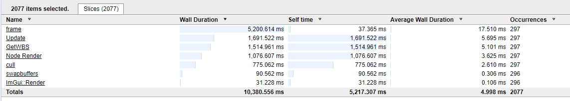
Once the changes are made, we verify that our code actually compiles and runs correctly before reprofiling. For reference, these are the old times from the instrumented profile:
Our new data layout gives us the following times:
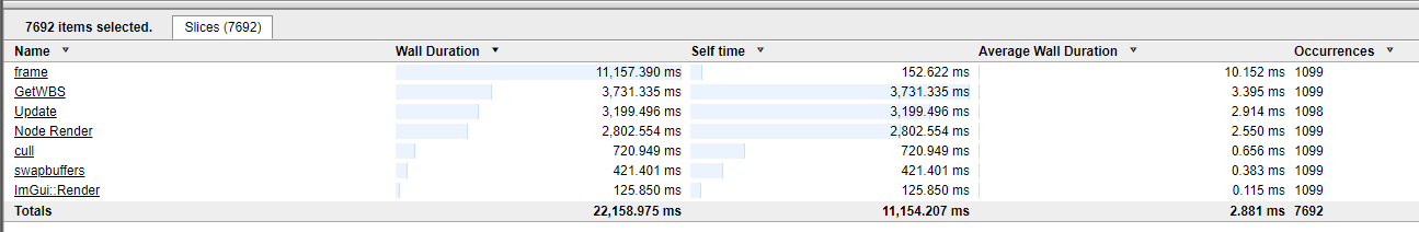
This means we’ve sped up our program from 17.5ms per frame to 10.15ms per frame! We’ve almost doubled the speed of the program just by changing the data layout.
If you learn just one thing from this set of articles, make sure it’s this: the layout of your data is a critical part of your program’s performance. People talk about the dangers of premature optimisation, but in my experience, a little forethought on how you structure your data relative to how you want to access and process it can make a dramatic difference in performance. If you’re unable to plan your data layout upfront, you should make every effort to write code that’s conducive to memory layout and usage refactors so that later optimisation is easier. In most cases, it isn’t your code that’s slow and needs to be refactored, it’s your data access.
The Next Bottleneck
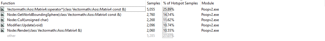
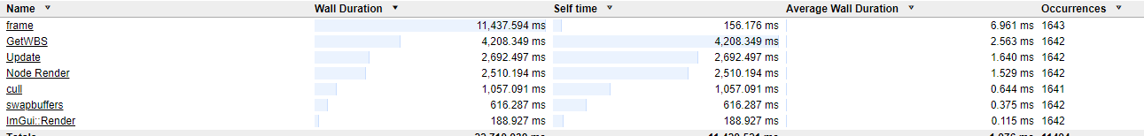
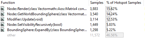
The code is faster now, but is it fast enough? Of course not. With the memory layout changes, the performance characteristics of the program have changed, so we’ll need to re-profile to find the next spot to optimise. Comparing the sampling profile runs we see the following:
Becomes:
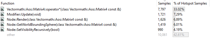
Notice that the sampling profile output doesn’t tell us whether the program is faster. All it tells us is the relative time spent in each function - in this case, more time is spent in the matrix operator multiply function after our changes. This doesn’t mean that that function is slower, only that more time is spent in this function relative to the others. Let’s have a look at the sample attribution now so we can see where the bottlenecks have moved to.
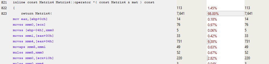
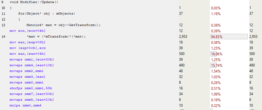
First, let’s look at Modifier::Update(). We can see that the matrix is no longer copied onto the stack. This makes sense as we’re passing in a pointer to a matrix now instead of copying an entire 64 byte matrix.
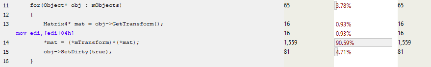
Most of the time in this function is spent in the setup for the function call to Matrix multiply and then in copying the result of that to the obj->mTransform location (truncated assembly below).

This begs the question: “How can we mitigate the cost of the function call?” The answer to that is simple, we just need to inline it. But if we look back at the Matrix multiply function we can see that it already has inline specified. So what’s going on here?
Compilers will often make decisions to automatically inline a function if it’s small enough, and you as the programmer have some control over that. You can change the maximum size of an inlined function, or some compilers will allow you to “force inline” a function, but there are costs to inlining. Code size can bloat and you can also begin to thrash your instruction cache if you’re executing more bytes of code from different locations.
Got SIMD?
The other thing we should notice about the Matrix multiply operator is that it’s using single floats - it’s not using SIMD (Single Instruction Multiple Data: modern CPUs provide instructions that can perform the same instruction on multiple instances of data, like multiply 4 floats at the same time). Even if we tell the compiler that we definitely want to use SIMD, it ignores us and generates code like this:
We’re not seeing SIMD instructions here because they require 16 byte aligned data - the data we have here is only 4 byte aligned. It’s possible to load unaligned data and then realign it into SIMD registers, but if we’re not doing very much SIMD processing, this can be slower than just doing it a single float at a time. Fortunately, we wrote the memory manager for these objects, so we can enforce 16 byte alignment (or even larger alignments) for our Matrices. For this example I’ve done just that. I’ve also forced the Vectormath library to generate only SIMD instructions.
Another profiling pass reveals an improvement. The average time for a frame drops from 10.15ms to around 7ms!
Looking at the sampling profile we see:
The first thing we notice is that the Matrix multiply operator has disappeared. What’s happened there is that the conversion to SIMD instructions has reduced the size of the function enough to allow the compiler to inline it - from 1060 bytes down to approx 350 bytes. The code for the matrix multiply has been included in each of the functions which call it, rather than those functions calling a single instance of the multiply function. As a side effect, code size increases (in this case the .exe went from 255kb to 256kb, so I’m not too worried about it) but we get the benefit of not requiring function parameters to be copied onto the stack for use by a called function.
Let’s look at Modifier::Update() in detail now:
Once again, we can see line 13 grabbing the pointer to the mTransform, and then almost immediately we can see the matrix SIMD code using the MOVAPS instruction (Move Aligned Single-Precision Floating-Point Values) to fill the xmm registers. So not only are we processing 4 floats at once with instructions like MULPS (Multiply Packed Single-Precision Floating-Point Values), we’re also loading in 4 floats at once, dramatically reducing the number of instructions in that function as well as improving its performance. Note that we do still suffer from stalls which can be attributed to cache misses, but our performance has improved here mainly due to better instruction usage and inlining. Since matrix multiply was called frequently, we’ve removed a significant amount of function call overhead.
In summary, we’ve optimised our frame time from 17.5ms down to around 7ms, speeding up our execution significantly without compromising our code in any way. We’ve made our code faster without adding significant complexity. We’ve added a constraint on how we allocate memory, but we can still make low-level changes without changing the high-level code.
Extra Credit: Virtual Functions
My original Pitfalls presentation went much further than I did here - it broke down the code, removing all the virtuals and adding a fair amount of code rigidity but improving the performance of the code by another factor of 2. I’m not going to do that - sure, we can hand optimise this example a lot further than we have, but at the expense of readability, extensibility, portability, and maintainability. What I will do is have a quick look at the implementation and impact of virtual functions.
Virtual functions are functions in a base class which can be redefined in derived classes. For example, we could have a Render() virtual function on our Object class and we could inherit from that to produce Cube() and Elephant() objects which define their own Render() functionality. We could add those new objects to one of our Nodes and when we call Render() on our generic Object pointer, the redefined Render() functions would be called, drawing a cube or elephant as appropriate.
The simplest test case in our example would be the SetVisibilityRecursively() method on Objects and Nodes. This method is used during the culling phase when a node is fully in or out of the frustum so all of its children can be trivially set to be visible or not. In the case of the Object, all it does is set an internal flag:
virtual void SetVisibilityRecursively(bool visibility)
{
    m_IsVisible = visibility;
}
The Node version does a little more, calling SetVisibilityRecursively() on all its children:
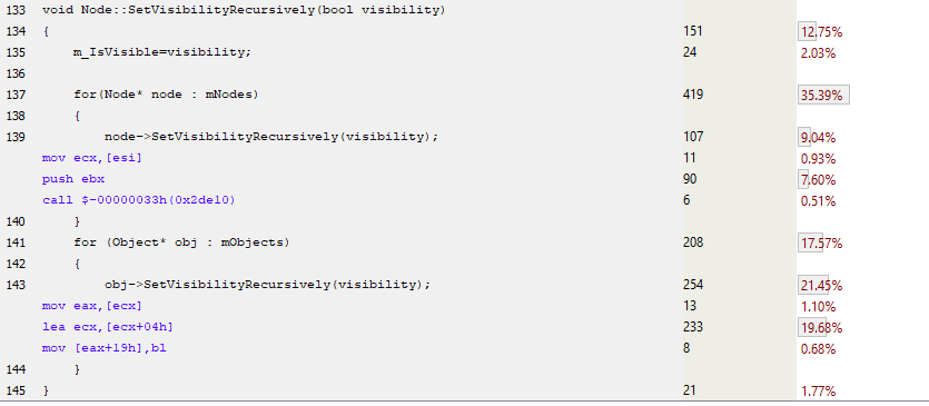
void Node::SetVisibilityRecursively(bool visibility)
{
    m_IsVisible = visibility;

    for(Object* obj : mObjects)
    {
    mObjects[i]->SetVisibilityRecursively(visibility);
    }
}
Looking at the sampling profile we see the following in the node version:
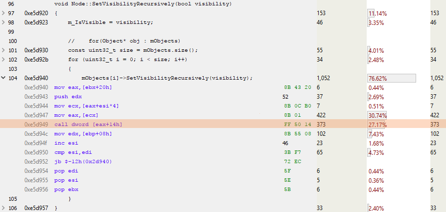
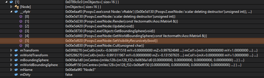
In this code, ESI is the counter for the loop and EAX is the pointer to the next object. The interesting bit in here is the CALL DWORD [EAX+14h] highlighted line - this line is calling the virtual function which is located 0x14 (20 decimal) bytes from the start of the virtual table. Since a pointer is 4 bytes and all sensible people count from zero, this is calling the 5th virtual function in the object vtable or, as we can see below, SetVisibilityRecursively():
As you can see, there is a little bit of extra work required when calling a virtual function. The vtable must be loaded and the virtual function must be looked up and then called, passing in any parameters as well as the “this” pointer.
Virtually no Virtuals
In the following sampled code, I have replaced the virtual functions in Nodes and Objects with normal functions. This means that I need to keep two arrays of things in each Node (Nodes and Objects) as they’re distinct from each other. The code below demonstrates this:
As you can see here, there are no virtual table loads and no virtual function dereferencing. We have a simple function call for the Node::SetVisibilityRecursively() implementation in the first case and the function is completely inlined in the second case for the Object implementation. Virtual functions can’t be inlined by the compiler as they can’t be determined at compile time, only during run time. So this non-virtual implementation looks like it should be faster. Let’s profile it and see for sure.

This optimisation has produced a very small change in performance, taking the frame time from 6.961ms to 6.963ms. Does this mean we’ve slowed down the code by 0.002ms? No, not at all. This time difference is well within the noise inherent in this system, the system in this case being a PC running an OS which is doing many other things at the same time (updating my Twitter feed, checking for new email, refreshing the animated gifs on a page I’d forgotten to close). To get an idea of the impact your OS has on the code you’re running, you can use a tool like the invaluable Windows Performance Analyser. This tool shows not just the performance of your code, but a holistic view of your entire system. So when your code suddenly takes twice as long to process, you can see if it was your fault or some other system hog stepping in and stealing your cycles. Check out Bruce Dawson’s excellent blog if this interests you.
What we’ve seen here is that the removal of virtuals had very little impact on the performance of our code. Even though we’re doing fewer virtual table lookups and executing fewer instructions, the program is still running at about the same speed. This is most likely due to the Wonders of Modern Hardware - branch prediction and speculative execution is good not just for hacking, but for taking your repetitive code and figuring out how to run it as fast as possible.
To quote Henry Petroski:
“The most amazing achievement of the computer software industry is its continuing cancellation of the steady and staggering gains made by the computer hardware industry.”
What I have shown here is not that the use of virtual functions is free, but rather that in the case of this code, the cost of virtual function use was negligible.
Summary
So far we’ve profiled our sample code, pinpointed some bottlenecks, and worked to minimise those bottlenecks. Every time we changed our code, we reprofiled it to see if we’d made it better or worse (mistakes are useful - we learn from them), and at each stage we understood the code, the way it executed, and the way it accessed memory a little better. The solution we settled on made minimal changes to the high-level code and decreased the amount of time it took to render a single frame from 17ms to 7ms. What we learnt was that memory is slow, and to write fast code we need to work with the hardware.
I hope you’ve enjoyed part two of this trip further down the performance rabbit hole and picked up a pointer or two that might help you with your own optimisations in the future. For part three of this series I’ll be looking at the detection, analysis, and optimisation of some recent performance bottlenecks that we’ve found in League itself. I hope you’ll join me for that.

For more information, check out the rest of this series:
Part 1: Measurement and Analysis
Part 2: Optimisation (this article)
Part 3: Real World Performance in League